Bayesian Model Selection & Scaling Laws
Why proxy-scale winners can lose at target scale: a Bayesian view of loss curves shows when to select for endpoint, cumulative, or warm-start performance.
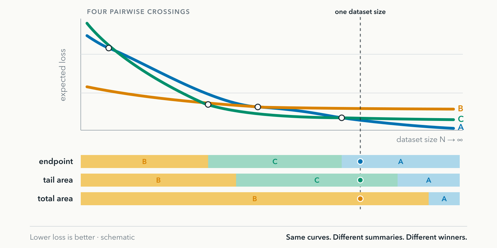
TL;DR. Scaling laws tell us how models improve with scale, but not what “best” should mean. Bayesian model-comparison criteria make a hidden choice visible: should we select the model with the best final checkpoint, the best cumulative performance while learning, or the best performance after a warm start? For an ideal Bayesian learner, these are the final height, total area, and tail area of its loss curve (dataset size vs loss): posterior-predictive loss, negative log marginal likelihood, and negative CLML. These criteria can rank the same models differently whenever the loss curves cross, which is why a proxy-scale winner may lose at target scale. Similar considerations apply to pretraining and in-context learning, even though the underlying models are usually not Bayesian. In general, the selection criterion should follow the downstream use case, not convention.
Two Loss Curves, Two Criteria
Let’s compare how the Bayesian view on model selection differs from how we usually treat model selection during pretraining (where by model selection I mean the process of selecting the preferred model from a set of models).
Imagine two single-pass pretraining runs on the same ordered data, matched except for one controlled change. Run A’s loss falls quickly but plateaus high. Run B starts higher, improves for longer, and finishes lower.
If you care about the final checkpoint, you pick B.
With equal prior probabilities over the candidate models, classical Bayesian model selection instead prefers the model with higher evidence, or equivalently lower negative log marginal likelihood, which essentially is the area under the loss curve. The closest analogue for an ordinary training run is the token- or example-weighted sum of first-pass losses on fresh batches, measured before updating on each batch. This is a prequential score for the training pipeline (generally not Bayesian evidence). Under this area criterion, B’s poor start remains part of the score and may outweigh its lower final loss: the area favours B only if its later advantage offsets its early deficit. Otherwise, final height and total area rank the runs differently.
In this post, we compare three criteria of an expected Bayesian loss curve: total area (expected negative log marginal likelihood), final height (posterior-predictive loss, estimated by validation or leave-one-out evaluation), and tail area (expected negative CLML). Their rankings depend on curve crossings, which in turn reflect differences in starting loss, loss floor, and descent rate. These features connect to prior-data conflict, model misspecification, and model complexity, respectively, and are also what pretraining scaling laws examine when they plot loss against the number of training tokens.
This post is an LLM-assisted rewrite, with substantial manual editing, of my ICLR 2024 blog post. The original developed the argument in information-theoretic notation; here I focus on loss curves in a more applied framing.
The Probability Chain Rule
Take a probabilistic model \(\mathcal{M}\) with a prior \(p(\theta \mid \mathcal{M})\) over its parameters and a likelihood \(p(x \mid \theta, \mathcal{M})\). The marginal likelihood, also called the evidence, integrates the parameters out:
\[ p(x_{1:N} \mid \mathcal{M}) = \int p(x_{1:N} \mid \theta, \mathcal{M}) \, p(\theta \mid \mathcal{M}) \, d\theta. \]
Bayes factors compare this quantity between two models. Empirical Bayes, also called type-II maximum likelihood, maximizes it over hyperparameters. In both roles, it appears to be a static score of how well a model explains a dataset.
We can use the chain rule to decompose it into sequential predictions:
\[ \log p(x_{1:N} \mid \mathcal{M}) = \sum_{n=1}^{N} \log p(x_n \mid x_{<n}, \mathcal{M}). \]
Each term is a posterior-predictive probability (or a density for continuous data). When data points are independent given the parameters,
\[ p(x_n \mid x_{<n}, \mathcal{M}) = \int p(x_n \mid \theta, \mathcal{M}) \, p(\theta \mid x_{<n}, \mathcal{M}) \, d\theta, \]
which is the evidence integral again, with the prior replaced by the posterior after the first \(n-1\) points. Write \(\ell_n = -\log p(x_n \mid x_{<n}, \mathcal{M})\) for this one-step-ahead loss. Then
\[ -\log p(x_{1:N} \mid \mathcal{M}) = \sum_{n=1}^{N} \ell_n. \]
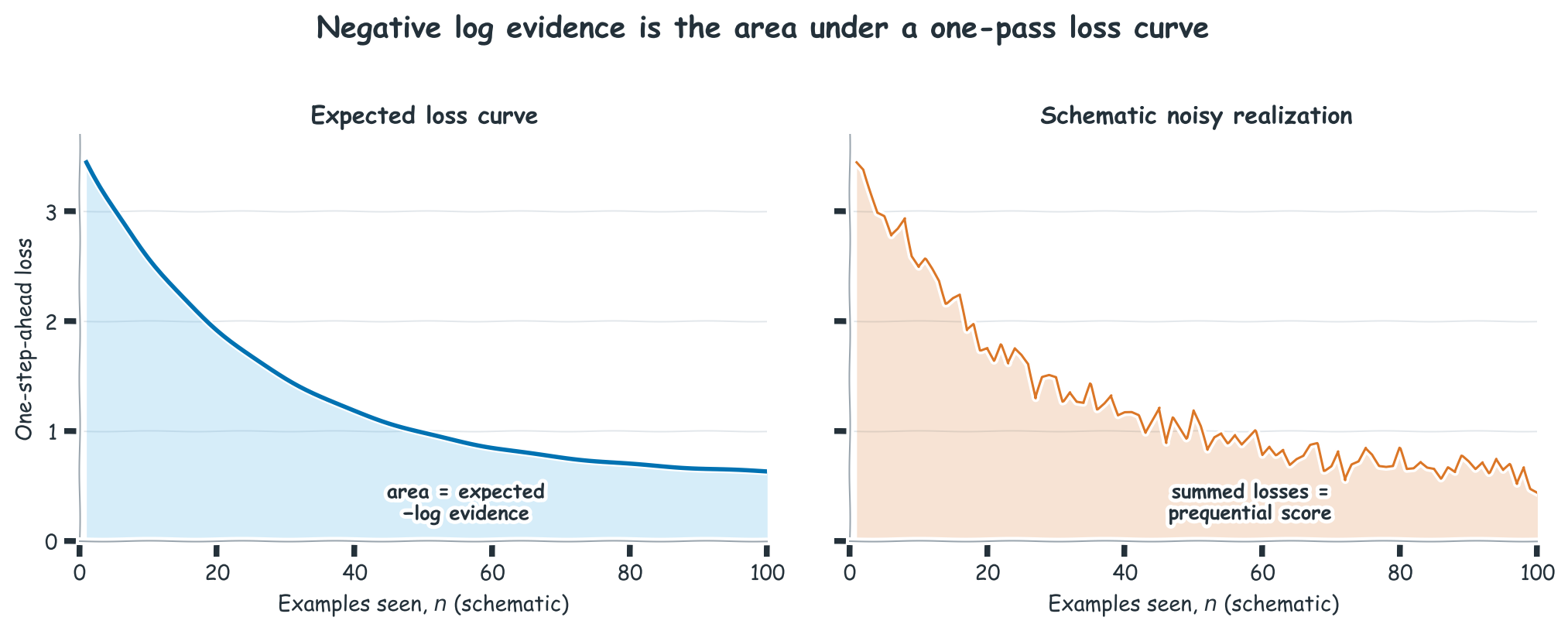
For a fixed dataset and order, the negative log evidence is therefore exactly the cumulative loss of an ideal Bayesian learner working through the data once. This learner updates by exact conditioning, not gradient descent. Plot the realized \(\ell_n\) against \(n\), and their area is the realized negative log evidence. Averaging over datasets or orderings gives the smooth expected loss curves used below; their area is the expected negative log evidence.
This has three implications:
First, the marginal likelihood is not determined by the final predictor alone. It scores the whole run. The first term is the prior-predictive loss on \(x_1\), so a poor prior retains that initial penalty even if the model eventually predicts well.
Second, the area is a code length. An arithmetic coder driven by these one-step-ahead predictions encodes discrete data in \(\sum_n \ell_n\) nats, up to coding overhead. This is the prequential (“predictive sequential”) view of model assessment introduced by the Bayesian statistician Philip Dawid in 1984: assess a forecasting system by the predictions it issued and the outcomes that followed. It is also the minimum-description-length reading of evidence. The same accounting turns a language model into a lossless compressor (Delétang et al., 2023), and prequential codes based on actual training runs give practical description lengths for deep networks (Blier & Ollivier, 2018). (Recently, Qiu et al. (2026) introduce a requential protocol, which can reconstruct a student model using substantially fewer bits, and compare it against prequential coding, whose code length is the sum of the model’s pre-update negative log probabilities on successive training batches.)
Third, first-pass SGD pretraining produces an analogous pre-update loss curve. Most tokens are seen once in modern pretraining, though curated subsets may be repeated (Muennighoff et al., 2023). Before an update uses a fresh batch, that batch is held out from the current parameters. The appropriately weighted sum of these losses is an exact prequential score for the specified training pipeline and ordered stream, but not generally an estimate of Bayesian evidence. In special settings, such as linear models and some infinite-width networks, sample-then-optimize procedures can generate posterior samples and thereby support Monte Carlo estimates or bounds for the evidence. However, a single ordinary SGD trajectory does not turn training loss into evidence.
Similarly, training-speed methods use different approximations. Lyle et al. (2020) derive marginal-likelihood lower-bound estimators under posterior-sampling constructions, whereas Ru et al. (2021) rank architectures by summed minibatch losses over early epochs. The latter is a heuristic training-curve area, not the exact one-pass identity above. These methods have been demonstrated to work well at neural-architecture-search scale (but not at frontier scale as far as I know).
The analogy between Bayesian log evidence curves and pretraining loss curves has two limits:
Area comparisons evaluate complete learners, not architectures in isolation. There is no unique way to split a finite SGD pipeline into a Bayesian prior and an inference procedure: architecture, parameterization, initialization, regularization, optimizer, and schedule jointly determine the curve. Two warmup or annealing schedules can produce very different areas yet similar final checkpoints. Comparing two complete learners is meaningful, but attributing the difference to architecture requires a matched training recipe. Final loss also depends on the stopping point and schedule.
For non-exchangeable learners such as SGD, area also depends on data order. A random reshuffle can change the area with little effect on final loss, and a deliberate curriculum can change both.
Three Ways to Read the Curve
The three model-selection criteria are computed from different parts of the curve:
| Functional of the curve | Bayesian name | Practical interpretation |
|---|---|---|
| Final height: expected next-point loss after conditioning on (nearly) all \(N\) points | posterior-predictive risk; averaged over held-out points and orderings, this becomes the leave-one-out cross-validation score | Bayesian model-averaged validation loss; ordinary checkpoint validation loss is analogous |
| Total area: \(\sum_{n=1}^{N} \ell_n\) | negative log marginal likelihood; negative log evidence | one-pass prequential score for a specified learner; training-speed proxy |
| Tail area: \(\sum_{n=N-k+1}^{N} \ell_n\) | negative conditional log marginal likelihood (CLML) | loss summed over the last \(k\) steps; analogous to suffix scoring in sliding-window perplexity |
Choosing the Criterion
We need to match the criterion to the deployment or scientific question. There is no single answer for which model is best.
Which fixed hypothesis explains the data? Use the total area. In hypothesis testing and Bayes factors, the prior is part of the hypothesis. Charging the model for its early predictions is the point. The marginal likelihood is the probability—or, for continuous data, density—the model assigned to the full dataset, and it composes sequentially. Under the standard tied-loss-floor asymptotics discussed below, its growing signal supports learning constraints, symmetries, and dimensionality. Gaussian-process empirical Bayes is a practical example because the marginal likelihood is differentiable and requires no validation split. MacKay’s chapter 28 gives the classic account. When the candidates are imperfect engineering alternatives rather than literal hypotheses, a predictive criterion is often more directly aligned with one’s goals, however.
Which frozen model generalizes best at the current data size? Use the final height. Validation loss or cross-validation estimates deployment risk when its data distribution, scoring rule, and effective training size match deployment. It is operationally straightforward, although very small endpoint gaps can require a large evaluation set to resolve.
Which learner predicts best while it keeps learning? Use an area, usually a tail area. In online learning, continual learning, sequential decision-making, and long ICL sessions, cumulative performance is what counts. If deployment starts from a warm state, discard the part of the curve before that state. Whole-stream compression, by contrast, needs the total area.
These are three members of a larger family of curve-weighting rules. A fixed deployment budget puts all weight on one endpoint; an uncertain stopping budget averages endpoints over the possible stopping points; a system used throughout adaptation weights the losses it incurs along the way; and a warm-start or discounted deployment downweights the beginning.
Can first-pass training loss replace held-out evaluation? Only as a pipeline-specific proxy. A running average of pre-update losses measures average online performance over the trajectory, not current-checkpoint performance. A sufficiently local window under slowly changing parameters can approximate the checkpoint’s loss on the training mixture. Training-stream areas from different mixtures score different distributions, so mixture selection still needs evaluation on a fixed target distribution. Per-token losses are also not directly comparable across tokenizers; they require a common unit, such as bits per byte, on the same underlying data. None of these quantities replaces fixed per-domain validation sets, of course. Training-speed estimators use the full area, so they retain the early losses. Scaling-law fits instead model the curve itself.
Conditional Marginal Likelihood as a Tail Area
The tail area is the negative of the conditional log marginal likelihood (CLML), which Lotfi et al. (2022), an ICML 2022 Outstanding Paper, proposed to address pathologies of the full marginal likelihood. It conditions on the first \(N-k\) points and scores only the remaining \(k\):
\[ \log p(x_{N-k+1:N} \mid x_{1:N-k}, \mathcal{M}) = \sum_{n=N-k+1}^{N} \log p(x_n \mid x_{<n}, \mathcal{M}). \]
It discards the beginning of the curve and scores only the tail. The tail size \(k\) therefore puts all three criteria in one family: \(k=N\) is the total area (negative log marginal likelihood), \(1<k<N\) is a proper tail area (negative CLML), and \(k=1\) is one realized one-step-ahead loss. Under exchangeability, averaging the \(k=1\) score over the held-out point gives leave-one-out cross-validation and estimates final-height risk after training on \(N-1\) points. Averaged over data orderings, the general \(k\) score corresponds, up to score-sign convention, to the cumulative leave-\(p\)-out cross-validation score studied by Fong & Holmes (2020).
There is no general rule for choosing the split. Lotfi et al. use 80% for conditioning and 20% for scoring; Fong and Holmes discuss scoring the final 10–50%. Different splits can select different models in the finite data regime, as the toy experiment below demonstrates.
After normalizing by the number of scored points, the criteria reduce to endpoint loss, full-run mean loss, and tail mean loss. For two models evaluated on the same realized data and order a strict ranking reversal between these positive-weight summaries requires the curves to cross.
When the Criteria Agree
Let \(L_n(\mathcal{M}) = \mathbb{E}[-\log p(X_{n+1}\mid X_{1:n},\mathcal{M})]\) denote the expected posterior-predictive loss, averaging over the training sample and a fresh point. Under the usual concentration assumptions, \(L_n\) approaches the best achievable predictor in the model class as n increases.
The expected endpoint and the normalized expected total and tail scores (where we divide by \(N\)) all converge to this loss floor. If two models have different loss floors, enough data makes their expected rankings agree. Empirical endpoint and tail rankings also require enough scored points for sampling noise to vanish.
In the standard asymptotics, a realizable
The exception is equal loss floors. Whether two LLM candidates have genuinely equal floors is difficult to determine from finite-range fits; such ties are nevertheless central to many traditional uses of Bayesian model selection.
With equal loss floors, the comparison comes down to the \(1/n\) terms. Suppose two nested models that contain the truth satisfy \(L_n^{(1)} = L_\infty + \lambda_1/n + o(1/n)\) and \(L_n^{(2)} = L_\infty + \lambda_2/n + o(1/n)\), with \(\lambda_1 < \lambda_2\). Their expected one-step-loss gap is asymptotically \(\Delta\lambda/n\), where \(\Delta\lambda = \lambda_2-\lambda_1\). The expected endpoint gap is therefore \(O(1/N)\) and can disappear into evaluation noise. Indeed, leave-one-out cross-validation is inconsistent for selecting the true model among nested linear models (Shao, 1993). The total-area gap satisfies \(\sum_{n \le N}\Delta\lambda/n \approx \Delta\lambda\log N\) and grows without bound, so the evidence can consistently prefer the simpler model. This is how marginal likelihood recovers the true dimensionality in Bayesian PCA and detects exact symmetries and constraints that are hard to see in held-out loss (Lotfi et al., 2022). A tail over a fixed fraction of the data has only a constant expected gap: scoring the last half gives \(\sum_{N/2 < n \le N}\Delta\lambda/n \approx \Delta\lambda\log 2\).
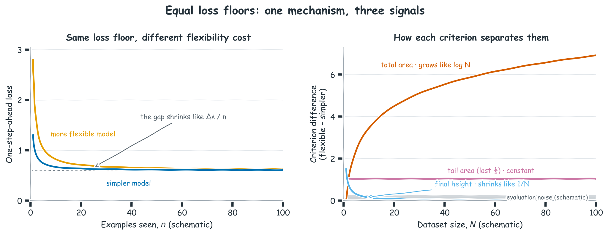
Different loss floors imply eventual agreement in expectation. Under the equal-loss-floor \(1/n\) asymptotics above, only the full area’s signal grows, while the signal of other criteria might also be lost to noise. LLM pretraining usually stops while loss is still falling, so practical comparisons remain in the finite-data regime where the criteria can disagree.
When the Criteria Disagree
A strict reversal of rankings by different criteria requires the loss curves to cross. Three regimes help explain those crossings: the long-run loss floor, the leading asymptotic approach to that floor, and the prior-sensitive finite-data behavior before that approximation becomes accurate.
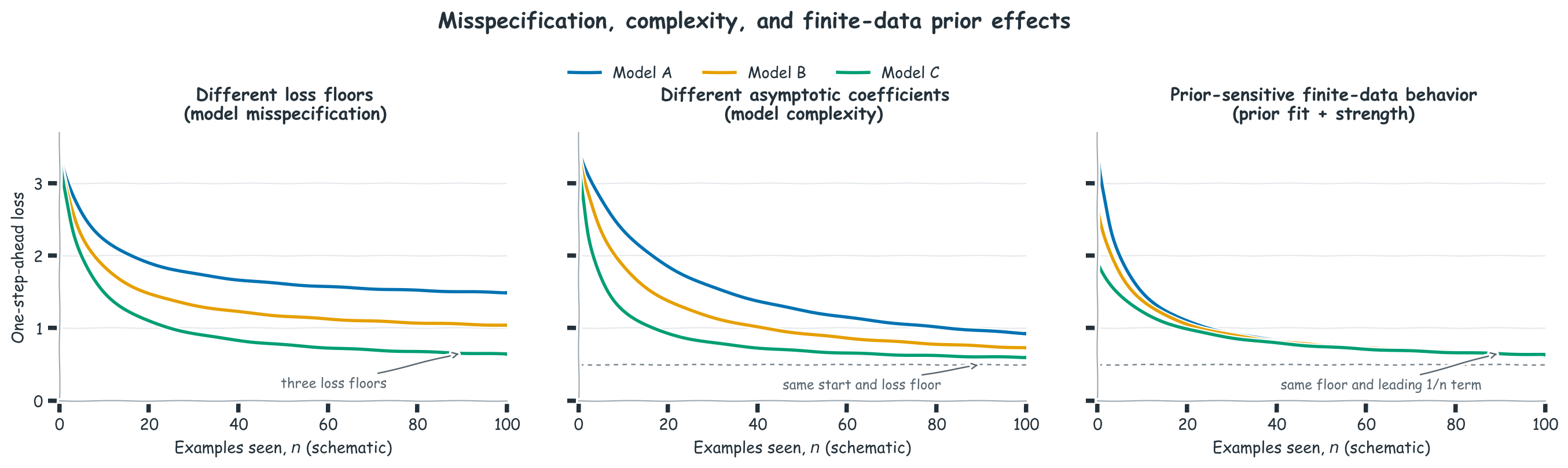
Model misspecification sets the excess loss floor. Under log loss and posterior concentration, the floor is the data entropy plus the minimum KL divergence from the data distribution to the prior-supported model class. This gap is zero when the truth is adequately supported and positive under misspecification. It is the relevant degree of misspecification here: a bounded context or a fixed recurrent state can leave a gap that no supported parameter setting closes. At large enough data scale, the model with the lower loss floor wins.
Model complexity controls the leading asymptotic descent in the realizable Bayesian settings above. The excess loss is \(d/(2n)\) for regular models and \(\lambda/n\) for singular models. The learning coefficient \(\lambda\) depends on the model, data-generating distribution, and prior; it is an effective asymptotic coefficient, not a generic measure of flexibility. Larger coefficients imply larger asymptotic excess losses and logarithmic evidence penalties, but do not determine finite-data or SGD descent. The Gaussian comparison below makes that boundary explicit: both models have \(d=1\) and hence the same leading \(1/(2n)\) excess, yet their early curves descend at very different local rates because prior-dependent finite-sample terms still matter. The coefficient \(d/2\) is already determined, but the low-data curve is simply not yet well described by this asymptotic term. For SGD, parameterization, optimization, the learning-rate schedule, and data order also shape the descent.
Prior-predictive fit and prior strength determine the finite-data regime, that is the starting loss and initial descent. A poor match between prior and data can arise from prior-data conflict, a prior placing most of its mass on parameter values contradicted by the data (Evans & Moshonov, 2006), but also from a diffuse prior whose predictions are simply too dispersed. A diffuse prior spreads its probability mass over a large parameter volume, leaving relatively little mass near the parameters that fit the data. Because marginal likelihood averages likelihood under the prior, this can lower the evidence even when posterior prediction later becomes good. This prior-volume effect is distinct from prior-data conflict.
How long a prior’s effect persists depends on its concentration (or effective sample size), its alignment with the likelihood, and the likelihood’s local geometry. A diffuse prior may start poorly but wash out quickly, whereas a concentrated conflicting prior can distort predictions for many updates. The starting loss alone therefore does not diagnose the mechanism.
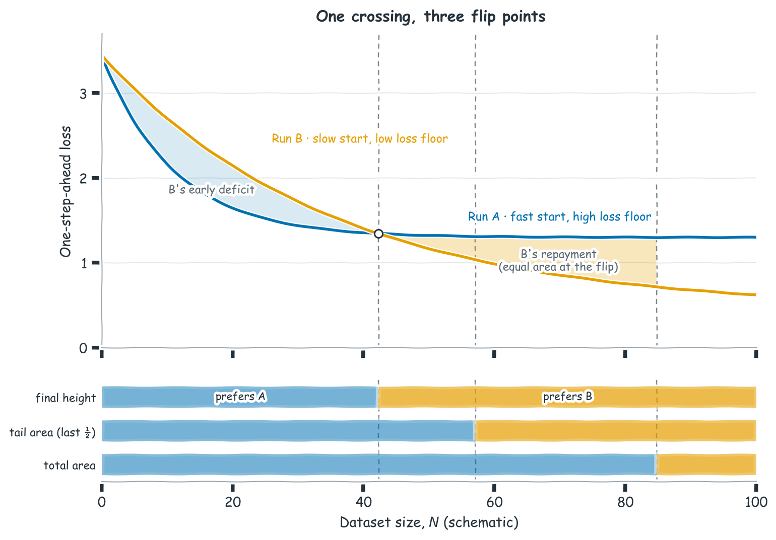
If one curve stays below the other everywhere, all three criteria give the same ranking. The classic crossing is the pattern from the introduction: Run A starts lower or descends faster but reaches a high loss floor, while Run B starts higher or descends more slowly and ends lower. Local optimization dynamics or shifts in the data stream can also produce crossings and re-crossings, so starting loss, loss floor, and asymptotic descent are useful but incomplete descriptors.
Suppose the curves cross, with B eventually dipping below A:
- The ranking by final height flips at every crossing. B becomes the better checkpoint the moment its curve passes below A’s.
- The ranking by total area flips only once B’s accumulated post-crossing advantage exceeds its earlier deficit. With a single crossing, this happens later, if it happens at all.
- The ranking by tail area depends on the split. For a fixed-fraction tail and one crossing, its flip point—if all three flip points exist—falls between the other two on the dataset-size axis. With multiple crossings, no such ordering is guaranteed.
Lotfi et al. observe a related non-monotonic relationship between marginal likelihood and generalization as dataset size changes: a good prior can dominate at very small \(N\), accumulated early losses can hurt at intermediate \(N\), and a lower loss floor eventually dominates.
Examples. A data-scaling law has the same geometry as the Bayesian learning curve, but it is not in general the same empirical curve. The Bayesian curve tracks one learner’s expected one-step loss after \(D\) examples. A scaling-law study usually trains a separate model at each data or compute budget and records final losses. For the ideal Bayesian construction, the two coincide in expectation. For SGD they need not: a checkpoint partway through one run need not match a separate run trained to that budget, especially under a decaying learning-rate schedule.
The Bayesian sum is specifically over sequential observations. It is not the visually shaded area under an arbitrary scaling-law plot: changing the horizontal axis from examples to log examples, tokens, FLOPs, time, energy, or money changes the weighting and therefore the question. An area per example and an area per FLOP can rank candidates differently when their cost per example differs. The exact identity above principally concerns data scaling; compute scaling shares the crossing geometry, but not the evidence interpretation.
In the standard fit \(L(D)=E+A D^{-\alpha}\), \(E\) is the fitted asymptote (loss floor), while \(A\) and \(\alpha\) describe the amplitude and rate of descent over the fitted range.
Prior-predictive fit and prior strength (starting loss and initial descent). Output-bias initialization in LLMs gives a concrete SGD analogue: the initialization induces an initial predictive distribution, which plays the role of the prior predictive. When the final-layer weights initially contribute negligible logits, zero token biases imply a uniform prediction, while random biases can induce an arbitrary distribution. Following Karpathy’s (2019) general initialization advice, Meister et al. (2023) make the language-model version explicit: setting each output bias to the log frequency of its token aligns the untrained model with the corpus’s unigram distribution.
Model misspecification and model complexity (loss floor and descent). Architecture-scaling studies usually mix these effects. At fixed model size, the \(D\to\infty\) loss floor includes the model class’s approximation gap; when model size also grows, the same gap may instead shrink as a parameter-scaling term. A reliably different asymptote under matched data and optimization would therefore be evidence of different degrees of misspecification, but finite-range fits often cannot identify it separately from the descent. A controlled comparison of transformers, recurrent models, and hybrids illustrates the problem: Merrill et al. (2026) find a robustly lower data-scaling coefficient for the hybrid, while differences in the fitted asymptote are not statistically conclusive.
Scaling studies nevertheless report several crossovers associated with model size and architecture. Architectures that match the transformer at small scale can fall behind as compute grows (Tay et al., 2022). The compute-optimal frontier is built from the same mechanism: plotted against compute, a small model can beat a large one early and lose later. The pareto frontier is the lower envelope of a family of such curves (Kaplan et al., 2020).
Optimization obviously also affects the loss curves: Xiao (2024) documents crossovers between constant and decaying learning rates and between weight-decay schedules, calling the phenomenon a scaling law crossover. Under a warmup–stable–decay schedule, the loss drops sharply only once the final decay starts, falling to match or undercut a cosine run of the same length (Hu et al., 2024; Hägele et al., 2024). In a matched benchmark of pretraining optimizers, loss curves cross during the decay phase, and rankings taken at intermediate checkpoints can reverse by the end of the run (Wen et al., 2025).
Nor is descent controlled by architecture and optimization alone. In controlled experiments, Mayilvahanan et al. (2025) find that pretraining data shapes loss-to-loss scaling (how loss on one dataset or task maps onto loss on another) far more than model size, optimizer, tokenizer, or even a Llama-versus-Mamba swap. Ye et al. (2025) find that the ranking of 20 pretraining mixtures shifts with model size and training duration, and in vision-language training, aggressive data filtering wins at small compute budgets and loses at large ones (Goyal et al., 2024). A data mixture that wins at proxy scale need not win at the target scale.
Finally note that if you extrapolate a crossing from fitted curves, you need to report uncertainty in its location. Choshen et al. (2025) analyse more than 1,000 scaling-law fits: intermediate checkpoints help, but seed variation and distance from the target scale still matter. Their results support using several runs or model sizes and excluding the unstable initial phase of training from the fit. A constant learning rate with short cooldown branches can recover an approximate endpoint at every intermediate budget from a single run (Hägele et al., 2024).
A Toy Experiment Where the Criteria Disagree
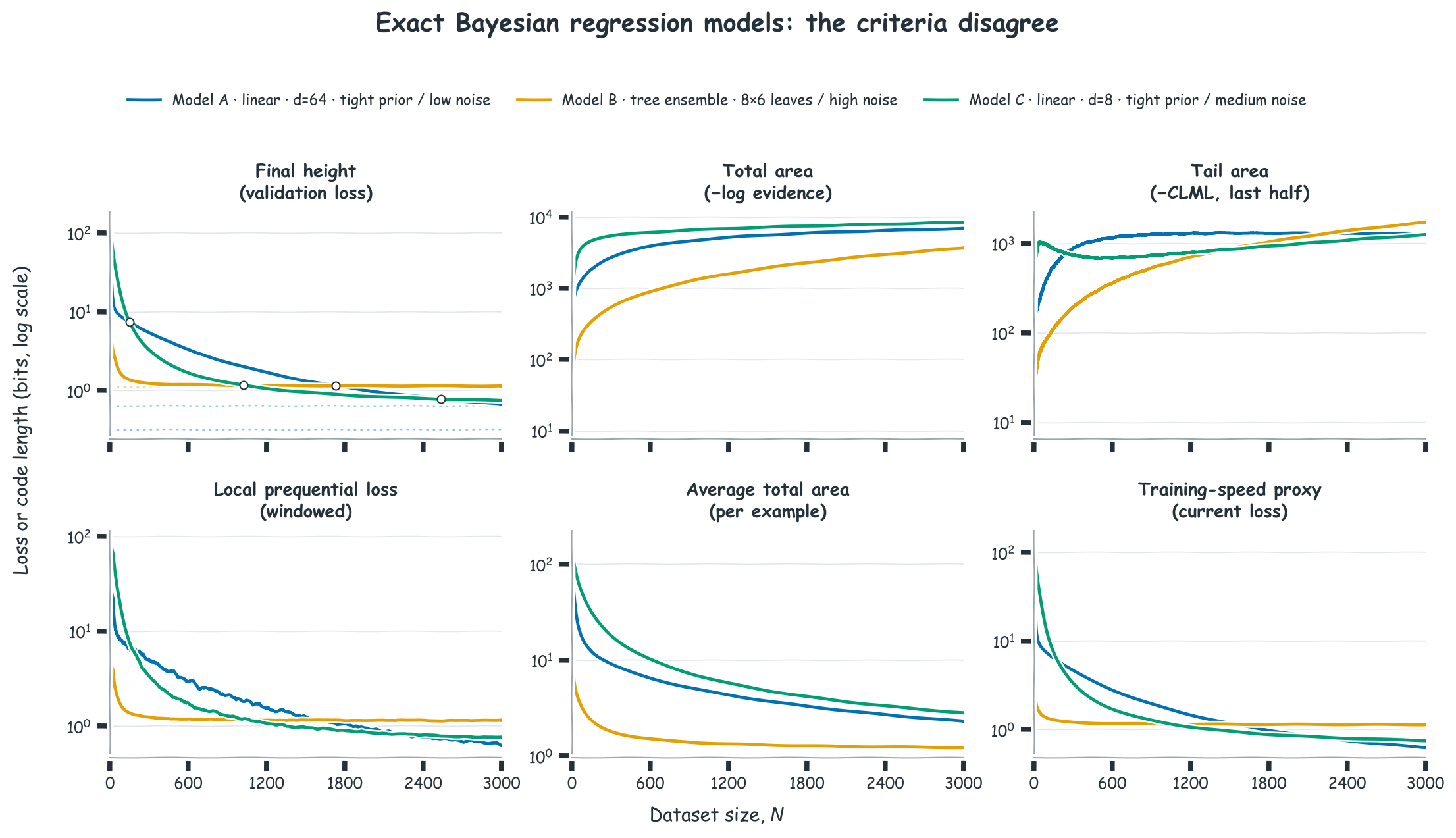
Conjugate Gaussian regression already produces this disagreement with exact posteriors and evidence. The target is a noiseless linear function of the first 8 of 64 independent uniform inputs. To make the learning curves visibly different, the candidates use two feature families:
- Model A: Bayesian linear regression on all 64 inputs, with coefficient-prior variance \(\phi=0.005\) and assumed noise \(\sigma_\text{noise}=0.5\);
- Model B: a fixed additive regression-tree ensemble on the 8 signal inputs, with 6 equal-width leaves per input, leaf-weight prior variance \(\phi=5\), and assumed noise \(\sigma_\text{noise}=0.8\);
- Model C: Bayesian linear regression on only the 8 signal inputs, with \(\phi=0.005\) and \(\sigma_\text{noise}=0.625\).
A and C therefore contain the true regression mean, while B can represent only a piecewise-constant approximation within its fixed leaves. B is not a conventionally fitted random forest: learning data-dependent splits would forfeit the conjugate marginal likelihood used here. It is a fixed tree feature map with Gaussian leaf weights, which retains exact evidence while giving the intended fast fit and approximation plateau.
The candidates deliberately vary all three ingredients. Their one-observation validation losses are about \(108\), \(10.5\), and \(136\) bits for A, B, and C; their population loss floors are \(0.33\), \(1.13\), and \(0.65\) bits. A has 64 linear coefficients, including 56 nuisance directions; B has 48 leaf weights (a 41-dimensional function space because the per-tree intercepts are redundant); C has 8 coefficients. The resulting validation curves have four well-separated pairwise crossings: A and C near \(N=150\), B and C near \(N=1{,}025\), A and B near \(N=1{,}730\), and A and C again near \(N=2{,}535\). The latter three are about 700 and 800 observations apart. Their lower envelope follows B \(\rightarrow\) C \(\rightarrow\) A. Because prior, model class, dimension, and assumed noise vary together, the experiment demonstrates criterion disagreement rather than assigning it to a single factor.
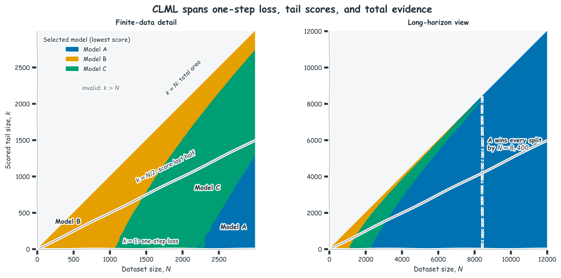
Varying dataset size \(N\) and scored tail size \(k\) together on a line shows which model minimizes a given tail ratio over time. A vertical slice through the next figure compares every criterion at one data scale: its bottom edge is the one-step score, its diagonal is the full marginal likelihood, and points between them are CLML with different splits.
The posterior, marginal likelihood, and CLML are computed exactly conditional on each split; their plotted averages and held-out losses remain finite-sample estimates. Only the training-speed curve additionally approximates its target. The selected model still varies with dataset size and split because the criteria measure different quantities, not because Bayesian inference is approximate. (Code and figure generation: local script. Original notebooks: toy experiment, visualizations.)
This disagreement is a finite-horizon effect, not a permanent inconsistency. A has the uniquely lowest population loss floor, so as \(N\) grows the endpoint, total-area, and every tail-area criterion all prefer A in expectation. Its endpoint eventually lies below the others; sufficiently late tails contain only that advantage, and in the full-area score it eventually outweighs the accumulated early deficit. The long-horizon panel of Figure 7 shows agreement across all splits by about \(N=8{,}400\). Realized rankings can still disagree because of sampling noise—especially for endpoint or short-tail scores—unless enough fresh observations are scored.
In-Context Learning with Frozen Weights
Finally, the chain-rule identity does not require parameter updates. For a fixed serialization of a prompt, a frozen autoregressive language model defines
\[ p(z_{1:T})=\prod_{t=1}^{T}p(z_t\mid z_{<t}), \]
so the negative log-probability of the ordered prompt is the sum of its token losses.
After choosing which tokens to score, sum their losses within each demonstration to form an in-context learning curve. Kaplan et al. (2020) plotted the related per-token loss against context position: LSTM curves plateaued early, while transformer curves kept falling. Relatedly, fixed-state architectures can remain competitive in average perplexity while being limited at copying and retrieval from long contexts (Jelassi et al., 2024).
Some ICL curves do invite a Bayesian reading: the pretrained model acts as a prior over tasks, and each demonstration is one more observation (Ortega et al., 2019; Xie et al., 2021). Prior-data fitted networks (models meta-trained on synthetic tasks drawn from a prior so that a forward pass mimics the posterior predictive) implement this by construction (Müller et al., 2022). For an ordinary pretrained LLM, however, calling the area under an ICL curve a task-level marginal likelihood assumes that its predictions correspond to coherent Bayesian conditioning over exchangeable examples.
The evidence for that stronger claim is mixed. Falck et al. (2024) find violations of a martingale property that any Bayesian learner must satisfy on exchangeable data: roughly, its predictions must not drift in expectation as it conditions on more data sampled from those same predictions. Arora et al. (2025) fit Bayesian scaling laws to real ICL curves and recover interpretable parameters, but non-Bayesian laws fit about as well. They present the Bayesian account as compatible with their results, not established by them.
The choice of score matters even without a Bayesian interpretation:
- Few-shot evaluation estimates expected query loss after a fixed number of demonstrations: a final-height criterion at the deployment shot count.
- Scoring the whole demonstration sequence is an area criterion. It includes zero-shot and one-shot performance even if the deployed prompt will always contain many examples.
- Discarding early positions before averaging produces a tail score analogous to CLML. Sliding-window perplexity does this when it scores only the final tokens of each overlapping window. The windows are not Bayesian tasks, but both criteria score only a tail.
If one model is better zero-shot and another adapts faster, their ICL curves may cross, causing the final-height, total-area, and tail-area criteria to rank them differently. For fixed-shot prompting, the relevant quantity is expected query loss at the deployment shot count. A long session in which cumulative performance matters calls for an area, perhaps with a warm-up period discarded.
Not every comparison produces a crossing. Marinescu et al. (2026) vary class-label representations and the number of demonstrations. Representation quality largely sets zero-shot accuracy and also affects the rate of improvement, but the ranking of label sets is mostly preserved across shot counts.
The curve need not even descend in a heterogeneous session. Li et al. (2026) derive and observe order-dependent interference and forgetting when several tasks share one prompt. A tail area can still measure cumulative session performance, but it then scores the task sequence as well as the model. One averaged ICL curve can hide negative transfer.
Occam’s Razor: No Silver Bullet
The marginal likelihood is often said to implement Occam’s razor automatically. A diffuse prior spreads prior-predictive probability over a broader set of possible datasets and therefore cannot assign high probability throughout that set. For fixed priors, this is a statement about distributions committed to before seeing the data; whether diffuseness lowers the evidence for a particular observed dataset depends on where that dataset lies.
But “prefer the shortest description” does not specify what must be described. Scoring only data fit gives the maximum-likelihood objective, though not by itself a complete code. Adding a finite-precision parameter code gives a two-part, MAP-like objective. A Bayesian mixture code for the full data stream gives negative log marginal likelihood; applying it only to a continuation gives negative CLML.
Which description is shortest depends on the prior, the code, and the prediction problem.
Estimating the Criteria in Deep Networks
For deep networks, approximation error in evidence or CLML estimates can exceed the between-model score differences of interest. Naive prior Monte Carlo has extreme relative variance because good parameter values occupy a tiny fraction of the prior. Common single-mode Laplace approximations and simple variational families can miss substantial posterior mass or modes.
I ran into this while reviewing the code for Lotfi et al. The first arXiv version accidentally computed the Bayesian-model-averaged validation loss (the validation loss of posterior-averaged predictions) in place of the CLML in its DNN experiment. Correcting the bug left the qualitative conclusions unchanged. For the CNNs, the Laplace-estimated CLML was also nearly indistinguishable from ordinary, non-model-averaged validation loss when I plotted their difference.
Takeaways
- For a fixed data order, negative log evidence is exactly the sum of realized Bayesian posterior-predictive losses; their expectation forms a smooth loss curve. Posterior-predictive validation or leave-one-out loss estimates its endpoint, and negative CLML is a tail sum.
- A strict ranking reversal requires crossing loss curves, so a proxy-scale winner can lose at target scale when it learns quickly but approaches a worse loss floor. If the floors are equal, scale does not reveal a different limiting-performance winner; instead, it changes how much model-selection signal each criterion accumulates: the endpoint gap shrinks as \(O(1/N)\), a fixed-fraction tail gap stays \(O(1)\), and the total-area gap grows as \(O(\log N)\). Evidence (total area) can therefore resolve an asymptotic complexity difference that endpoint or tail estimates may lose in evaluation noise.
- First-pass SGD loss is an exact prequential score for a specified ordered training pipeline, not generally an estimate of Bayesian evidence. Scaling laws obey the same crossing logic, but the meaning of an area depends on whether the horizontal measure is examples, tokens, compute, time, or cost. Fits should use multiple budgets and seeds, with uncertainty on any predicted crossing.
- A criterion is a weighting over learning states. Use the total area for fixed-prior hypothesis comparison and whole-stream compression, the final height for frozen deployment at a fixed budget, and a tail area when cumulative performance after a warm start matters.
- For In-Context Learning, the chain rule exactly decomposes negative log-probability into token losses. Reading their area as a Bayesian task marginal likelihood requires stronger assumptions about coherent task inference, and whole-prompt likelihood may measure formatting and input probability as much as adaptation.
Appendix: Terminology Map
For readers coming from the original post or the Bayesian literature: this post distinguishes realized self-information, \(-\log p(x_n\mid x_{<n})\), from its expectation. The original post’s entropy notation \(\mathrm{H}[\cdot]\) refers to expected quantities.
| This post | Literature / original post |
|---|---|
| realized one-step-ahead loss \(\ell_n\) | negative log posterior predictive; the expectation is conditional marginal information \(\mathrm{H}[X_n \mid X_{<n}, \mathcal{M}]\) |
| final height (expected) | conditional marginal cross-entropy; expected leave-one-out CV loss; held-out NLL |
| realized total area | negative log marginal likelihood; the expectation is joint marginal information; prequential code length |
| realized tail area | negative conditional log marginal likelihood (CLML, Lotfi et al., 2022); the expectation is conditional joint marginal information |
| tail area, averaged over orderings | cumulative leave-\(p\)-out CV score (Fong & Holmes, 2020); conditional joint marginal cross-entropy |
Acknowledgements: This post is a rewrite of my ICLR 2024 blog post, which grew out of an exchange with the authors of Lotfi et al. (2022). I thank them for their engagement, and Freddie Bickford Smith for comments on the original. LLM assistance was used in drafting and editing both versions.